Intermediate Python for Data Science
This notebook contains most of the essential elements of Python skill for data science. While you go through it, you will learn about
- how to use matplotlib to visualize data
- how to use pandas dataframe, read and manupulate data
- Dictionaries
- logic control flows
- loop
- Random walk - A case study.
Matplotlib
import numpy as np
import matplotlib.pyplot as plt
import pandas as pd
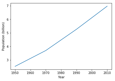
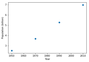
year = [1950, 1970, 1990, 2010]
pop = [2.519, 3.69, 5.263, 6.972]

# line plot
plt.plot(year, pop)
plt.xlabel("Year")
plt.ylabel("Population (billion)")
plt.show()
# Scatter PLot
plt.scatter(year, pop)
plt.xlabel("Year")
plt.ylabel("Population (billion)")
plt.show()
data = pd.read_csv("data/worldpop.csv")
data.head()
| Unnamed: 0 | country | year | population | cont | life_exp | gdp_cap | |
|---|---|---|---|---|---|---|---|
| 0 | 11 | Afghanistan | 2007 | 31889923.0 | Asia | 43.828 | 974.580338 |
| 1 | 23 | Albania | 2007 | 3600523.0 | Europe | 76.423 | 5937.029526 |
| 2 | 35 | Algeria | 2007 | 33333216.0 | Africa | 72.301 | 6223.367465 |
| 3 | 47 | Angola | 2007 | 12420476.0 | Africa | 42.731 | 4797.231267 |
| 4 | 59 | Argentina | 2007 | 40301927.0 | Americas | 75.320 | 12779.379640 |
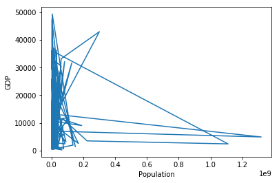
pop = data["population"]
gdp = data["gdp_cap"]
# Line PLot
plt.plot(pop, gdp)
plt.xlabel("Population")
plt.ylabel("GDP")
plt.show()
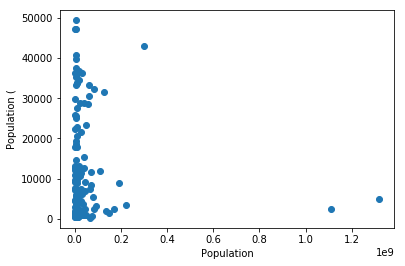
# Scatter PLot
plt.scatter(pop, gdp)
plt.xlabel("Population")
plt.ylabel("Population (")
plt.show()
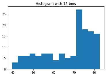
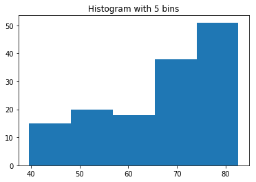
Histogram
life_exp = data["life_exp"]

plt.title("Histogram with 15 bins")
plt.hist(life_exp, bins=15)
plt.show()

# to clean up plot
plt.clf()


plt.title("Histogram with 5 bins")
plt.hist(life_exp, bins=5)
plt.show()
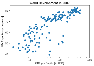
# basic scatter
# Scatter plot
plt.scatter(gdp, life_exp)

# Previous customizations
plt.xscale('log')
plt.xlabel('GDP per Capita [in USD]')
plt.ylabel('Life Expectancy [in years]')
plt.title('World Development in 2007')

# Definition of tick_val and tick_lab
tick_val = [1000, 10000, 100000]
tick_lab = ['1k', '10k', '100k']

# Adapt the ticks on the x-axis
plt.xticks(tick_val, tick_lab)

# After customizing, display the plot
plt.show()
Dictionaries and Pandas
# Definition of dictionary
europe = {'spain':'madrid', 'france':'paris', 'germany':'berlin', 'norway':'oslo' }

# Print out the keys in europe
print(europe.keys(), '\n')

# Print out value that belongs to key 'norway'
print(europe['norway'])
dict_keys(['spain', 'france', 'germany', 'norway'])

oslo
# Build cars DataFrame
names = ['United States', 'Australia', 'Japan', 'India', 'Russia', 'Morocco', 'Egypt']
dr =  [True, False, False, False, True, True, True]
cpc = [809, 731, 588, 18, 200, 70, 45]
dict = { 'country':names, 'drives_right':dr, 'cars_per_cap':cpc }
cars = pd.DataFrame(dict)
print(cars,"\n\n")

# Definition of row_labels
row_labels = ['US', 'AUS', 'JAP', 'IN', 'RU', 'MOR', 'EG']

# Specify row labels of cars
cars.index = row_labels

# Print cars again
print(cars)
         country  drives_right  cars_per_cap
0  United States          True           809
1      Australia         False           731
2          Japan         False           588
3          India         False            18
4         Russia          True           200
5        Morocco          True            70
6          Egypt          True            45


           country  drives_right  cars_per_cap
US   United States          True           809
AUS      Australia         False           731
JAP          Japan         False           588
IN           India         False            18
RU          Russia          True           200
MOR        Morocco          True            70
EG           Egypt          True            45
# to read data
brics = pd.read_csv("data/brics.csv", index_col = 0)

# to print data
print("Our brics dataset....\n")
print(brics, "\n\n")

# return pandas series
print("Printing pandas series...\n")
print(brics["country"], "\n\n")

# return pandas dataframe
print("Printing pandas dataframe...\n")
print(brics[["country"]],"\n\n")


# multiple dataframes
print("Printing multiple dataframes...\n")
print(brics[["country", "population"]],"\n\n")

# Multiple dataframes with index
print("Printing multiple dataframes with indexing...\n")
print(brics[1:4])
Our brics dataset....

         country    capital    area  population
BR        Brazil   Brasilia   8.516      200.40
RU        Russia     Moscow  17.100      143.50
IN         India  New Delhi   3.286     1252.00
CH         China    Beijing   9.597     1357.00
SA  South Africa   Pretoria   1.221       52.98


Printing pandas series...

BR          Brazil
RU          Russia
IN           India
CH           China
SA    South Africa
Name: country, dtype: object


Printing pandas dataframe...

         country
BR        Brazil
RU        Russia
IN         India
CH         China
SA  South Africa


Printing multiple dataframes...

         country  population
BR        Brazil      200.40
RU        Russia      143.50
IN         India     1252.00
CH         China     1357.00
SA  South Africa       52.98


Printing multiple dataframes with indexing...

   country    capital    area  population
RU  Russia     Moscow  17.100       143.5
IN   India  New Delhi   3.286      1252.0
CH   China    Beijing   9.597      1357.0
# Row access: loc
print("Row access pandas series\n")
print(brics.loc["IN"],"\n\n")

print("Row access pandas dataframe\n")
print(brics.loc[["IN"]],"\n\n")

print("Multple Row access\n")
print(brics.loc[["IN", "CH", "SA"]],"\n\n")

print("Rows with specific column\n")
print(brics.loc[["RU", "IN","SA"], ["country", "capital"]])
Row access pandas series

country           India
capital       New Delhi
area              3.286
population         1252
Name: IN, dtype: object


Row access pandas dataframe

   country    capital   area  population
IN   India  New Delhi  3.286      1252.0


Multple Row access

         country    capital   area  population
IN         India  New Delhi  3.286     1252.00
CH         China    Beijing  9.597     1357.00
SA  South Africa   Pretoria  1.221       52.98


Rows with specific column

         country    capital
RU        Russia     Moscow
IN         India  New Delhi
SA  South Africa   Pretoria
# iloc

print("Row access pandas dataframe\n")
print(brics.iloc[[1]],"\n\n")

print("Multple Row access\n")
print(brics.iloc[[1, 2, 4]],"\n\n")

print("Rows with specific column\n")
print(brics.iloc[[1, 2, 4], :3])
Row access pandas dataframe

   country capital  area  population
RU  Russia  Moscow  17.1       143.5


Multple Row access

         country    capital    area  population
RU        Russia     Moscow  17.100      143.50
IN         India  New Delhi   3.286     1252.00
SA  South Africa   Pretoria   1.221       52.98


Rows with specific column

         country    capital    area
RU        Russia     Moscow  17.100
IN         India  New Delhi   3.286
SA  South Africa   Pretoria   1.221
Logic Control flow and filtering
my_house = np.array([18.0, 20.0, 10.75, 9.50])
your_house = np.array([14.0, 24.0, 14.25, 9.0])

# my_house greater than 18.5 or smaller than 10
print(np.logical_or(my_house > 18.5, my_house < 10))

# Both my_house and your_house smaller than 11

print(np.logical_and(my_house < 11, your_house < 11))
print(my_house)
[False  True False  True]
[False False False  True]
[18.   20.   10.75  9.5 ]
cars = pd.read_csv('data/cars.csv', index_col = 0)

# Extract drives_right column as Series: dr
dr = cars["drives_right"]

# Use dr to subset cars: sel
sel = cars[dr]

# Print sel
print(sel)
     cars_per_cap        country  drives_right
US            809  United States          True
RU            200         Russia          True
MOR            70        Morocco          True
EG             45          Egypt          True
# Create car_maniac: observations that have a cars_per_cap over 500
cpc = cars['cars_per_cap']
car_maniac = cpc > 500
print("Cars dataset more than 500 cars ..\n\n",cars[car_maniac])
Cars dataset more than 500 cars ..

      cars_per_cap        country  drives_right
US            809  United States          True
AUS           731      Australia         False
JAP           588          Japan         False
between = np.logical_and(cpc > 100, cpc < 500)
medium = cars[between]
print("Cars dataset with cars between 100 and 500 cars per capital..\n\n", medium)
Cars dataset with cars between 100 and 500 cars per capital..

     cars_per_cap country  drives_right
RU           200  Russia          True
Loop
# while loop
x = 10
while x > 0:
    print("x is now: ", x)
    x = x - 2
x is now:  10
x is now:  8
x is now:  6
x is now:  4
x is now:  2
# for loop

# areas list
areas = [11.25, 18.0, 20.0, 10.75, 9.50]

for area in areas:
    print(area)

print("\nenumerate: looping with index\n")
for index, area in enumerate(areas):
    print("Area ", index, ": ", area)
11.25
18.0
20.0
10.75
9.5

enumerate: looping with index

Area  0 :  11.25
Area  1 :  18.0
Area  2 :  20.0
Area  3 :  10.75
Area  4 :  9.5
# house list of lists
house = [["hallway", 11.25],
         ["kitchen", 18.0],
         ["living room", 20.0],
         ["bedroom", 10.75],
         ["bathroom", 9.50]]

# Build a for loop from scratch

for room in house:
    print("the " + room[0] + " is " + str(room[1]) + " sqm" )
the hallway is 11.25 sqm
the kitchen is 18.0 sqm
the living room is 20.0 sqm
the bedroom is 10.75 sqm
the bathroom is 9.5 sqm
# iterate over dictionary

# Definition of dictionary
europe = {'spain':'madrid', 'france':'paris', 'germany':'berlin',
          'norway':'oslo', 'italy':'rome', 'poland':'warsaw', 'austria':'vienna' }

# Iterate over europe
for country, capital in europe.items():
    print("The capital of ", country, " is ", capital)
The capital of  spain  is  madrid
The capital of  france  is  paris
The capital of  germany  is  berlin
The capital of  norway  is  oslo
The capital of  italy  is  rome
The capital of  poland  is  warsaw
The capital of  austria  is  vienna
# looping over n dimensional numpy array

np_height = np.array([[23, 40, 55], [55, 90, 11]])

for height in np.nditer(np_height):
    print(height)
23
40
55
55
90
11
# looping over pandas dataframe

cars = pd.read_csv('data/cars.csv', index_col = 0)

# Iterate over rows of cars
for lab, row in cars.iterrows() :
    print(lab, ": ",row['cars_per_cap'] )
US :  809
AUS :  731
JAP :  588
IN :  18
RU :  200
MOR :  70
EG :  45
# adding new rows
cars["Name_lenght"] = cars['country'].apply(len)
print(cars)
     cars_per_cap        country  drives_right  Name_lenght
US            809  United States          True           13
AUS           731      Australia         False            9
JAP           588          Japan         False            5
IN             18          India         False            5
RU            200         Russia          True            6
MOR            70        Morocco          True            7
EG             45          Egypt          True            5
Case Study: Hacker Statistics
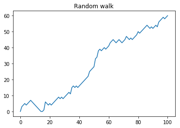
Random Walk
A random walk is a mathematical object, known as a stochastic or random process, that describes a path that consists of a succession of random steps on some mathematical space such as the integers.
np.random.seed(123)

random_walk = [0]

for x in range(100) :
    step = random_walk[-1]
    dice = np.random.randint(1,7)

    if dice <= 2:
        # Replace below: use max to make sure step can't go below 0
        step = max(0,step - 1)
    elif dice <= 5:
        step = max(0, step + 1)
    else:
        step = max(0, step + np.random.randint(1,7))

    random_walk.append(step)

print(random_walk)
[0, 3, 4, 5, 4, 5, 6, 7, 6, 5, 4, 3, 2, 1, 0, 0, 1, 6, 5, 4, 5, 4, 5, 6, 7, 8, 9, 8, 9, 8, 9, 10, 11, 12, 11, 15, 16, 15, 16, 15, 16, 17, 18, 19, 20, 21, 22, 25, 26, 27, 28, 33, 34, 38, 39, 38, 39, 40, 39, 40, 41, 43, 44, 45, 44, 43, 44, 45, 44, 43, 44, 45, 47, 46, 45, 46, 45, 46, 47, 48, 50, 49, 50, 51, 52, 53, 54, 53, 52, 53, 52, 53, 54, 53, 56, 57, 58, 59, 58, 59, 60]
# visualization random walk
plt.plot(random_walk)
plt.title("Random walk")
plt.show()
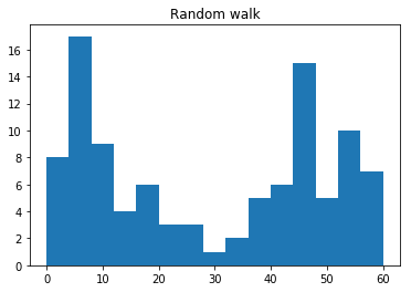
# visualization random walk
plt.hist(random_walk, bins = 15)
plt.title("Random walk")
plt.show()
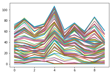
# Distribution

# initialize and populate all_walks
all_walks = []
for i in range(10) :
    random_walk = [0]
    for x in range(100) :
        step = random_walk[-1]
        dice = np.random.randint(1,7)
        if dice <= 2:
            step = max(0, step - 1)
        elif dice <= 5:
            step = step + 1
        else:
            step = step + np.random.randint(1,7)
        random_walk.append(step)
    all_walks.append(random_walk)

# Convert all_walks to Numpy array: np_aw
np_aw = np.array(all_walks)

# Plot np_aw and show
plt.plot(np_aw)
plt.show()

# Clear the figure
plt.clf()

# Transpose np_aw: np_aw_t
np_aw_t = np_aw.T

# Plot np_aw_t and show
plt.plot(np_aw_t)
plt.show()