Linear Regression from Scratch
Introduction
Statistical learning refers to a large collection of tools that are used for understanding data. Statistical learning can be divided into two categories which are called supervised learning and unsupervised learning.
Supervised Learning
In Supervised learning the dataset contains both input and it’s output, which means the output of given input data is known. Typically, the output need to be provided by a person or by another algorithm, that’s why it’s called supervised learning. In supervised learning if the output is quantitative, we call it regression problem. If the output is qualitative we call it Classification problem. Throughout the tutorial we will work with regression problem.
A linear regression typically looks like this:
where x is the input and y the output of given x. Beta_0 is randomly initialized and beta_1 comes from the given x [coefficient varience]. In the following we will try to generate x and y
Generating Example Regression data
import numpy as np
import scipy.stats as ss
import matplotlib.pyplot as plt
n = 100 # number of observation
beta_0 = 5
beta_1 = 3
np.random.seed(1)
x = 10 * ss.uniform.rvs(size=n)
y = beta_0 + beta_1 *x + ss.norm.rvs(loc=0, scale=1, size=n)
# Let's plot our generated data
plt.figure()
plt.plot(x,y, "o", ms=2)
xx =np.array([0, 10])
plt.plot(xx, beta_0 + beta_1 * xx)
plt.xlabel("x")
plt.ylabel("y")
Text(0,0.5,'y')
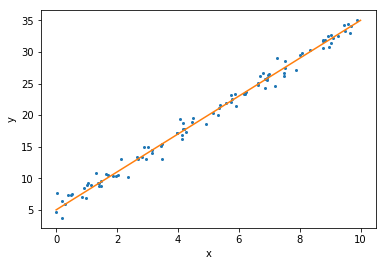
The orange line, the straight line here, is the function [beta_0 + beta_1 * xx] that we used to generate the data from. The blue dots here correspond to realizations from this model. So what we did was we first sampled 100 points from the interval 0 toto 10. Then we computed the corresponding y values. And then we added a little bit of normally distributed or Gaussian noise all of those points. And that’s why the points are being scattered around the line.
Residual Sum Square [RSS]
The residual for the observation is going to be given by the data point subtract from our predicted value for that same data point. which is as follows: So e sub i here is the difference between the i-th observed response value and the i-th response value predicted by the model. Now look below how we can compute the RSS in code.
Least Square Estimation in Code
rss = []
slopes = np.arange(-10, 15, 0.01)
for slope in slopes:
    rss.append(np.sum((y - beta_0 - slope * x)**2 ))

ind_min = np.argmin(rss)
print("Estimate for the slope: ", slopes[ind_min])
Estimate for the slope: 2.999999999999723
# Plotting RSS
plt.figure()
plt.plot(slopes, rss)
plt.xlabel("Slope")
plt.ylabel("RSS")
Text(0,0.5,'RSS')
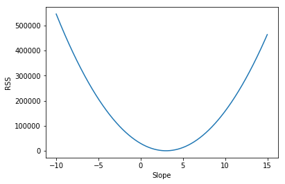
Here in the figure on the x-axis, we have the different slopes that we tried out from -10 to 15. On the y-axis, we have the different rss values. The goal is to find the value of slope, the value of the parameter that gives us the smallest value for RSS. And looking at the plot, it looks like it happens at around 3. If we go back to our Python code, we’ll see that our estimate was exactly 3.0 in this case.
Simple Linear Regression
Now that we have our x and y values. We can create a siimple linear regression model using statsmodels.api library. First we will try to create the model without intializing constant value, which is . As you can see from the output the standard error is 0.051 without constant.
import statsmodels.api as sm

mod = sm.OLS(y, x)
est = mod.fit()
print(est.summary())
                            OLS Regression Results
==============================================================================
Dep. Variable:                      y   R-squared:                       0.982
Model:                            OLS   Adj. R-squared:                  0.982
Method:                 Least Squares   F-statistic:                     5523.
Date:                Sat, 05 Jan 2019   Prob (F-statistic):           1.17e-88
Time:                        20:09:22   Log-Likelihood:                -246.89
No. Observations:                 100   AIC:                             495.8
Df Residuals:                      99   BIC:                             498.4
Df Model:                           1
Covariance Type:            nonrobust
==============================================================================
                 coef    std err          t      P>|t|      [0.025      0.975]
------------------------------------------------------------------------------
x1             3.7569      0.051     74.320      0.000       3.657       3.857
==============================================================================
Omnibus:                        7.901   Durbin-Watson:                   1.579
Prob(Omnibus):                  0.019   Jarque-Bera (JB):                3.386
Skew:                           0.139   Prob(JB):                        0.184
Kurtosis:                       2.143   Cond. No.                         1.00
==============================================================================

Warnings:
[1] Standard Errors assume that the covariance matrix of the errors is correctly specified.
X = sm.add_constant(x)
mod = sm.OLS(y, X)
est = mod.fit()
print(est.summary())
                            OLS Regression Results
==============================================================================
Dep. Variable:                      y   R-squared:                       0.990
Model:                            OLS   Adj. R-squared:                  0.990
Method:                 Least Squares   F-statistic:                     9359.
Date:                Sat, 05 Jan 2019   Prob (F-statistic):           4.64e-99
Time:                        20:09:22   Log-Likelihood:                -130.72
No. Observations:                 100   AIC:                             265.4
Df Residuals:                      98   BIC:                             270.7
Df Model:                           1
Covariance Type:            nonrobust
==============================================================================
                 coef    std err          t      P>|t|      [0.025      0.975]
------------------------------------------------------------------------------
const          5.2370      0.174     30.041      0.000       4.891       5.583
x1             2.9685      0.031     96.741      0.000       2.908       3.029
==============================================================================
Omnibus:                        2.308   Durbin-Watson:                   2.206
Prob(Omnibus):                  0.315   Jarque-Bera (JB):                1.753
Skew:                          -0.189   Prob(JB):                        0.416
Kurtosis:                       3.528   Cond. No.                         11.2
==============================================================================

Warnings:
[1] Standard Errors assume that the covariance matrix of the errors is correctly specified.
We added constant value and the standard error is now 0.031. Which is much smaller than before. That means model works better by initilizing beta_0 [ constant vlaue ]
Multiple Linear Regression
A multiple regression model with two inputs. The model predictions for the output are given by y
Generating data
n = 500
beta_0 = 5
beta_1 = 2
beta_2 = -1
np.random.seed(1)
x_1 = 10 * ss.uniform.rvs(size=n)
x_2 = 10 * ss.uniform.rvs(size=n)
y = beta_0 + beta_1 * x_1 + beta_2 * x_2 + ss.norm.rvs(loc=0, scale=1, size=n)

X = np.stack([x_1, x_2], axis=1)
To construct a capital X variable, the idea here is to take our x1 variable and our x2 variableand stack them as columns into a capital X variable, turning it into a matrix. So we can do this by using the np.stack function. So our input consists of a list (x1, x2) where we specify the vectors, or arrays, that we would like to stack. Then we also have to specify the axis. Remember this starts from 0. And because we would like exponent x to be columns in this matrix, we will use axis equals 1.
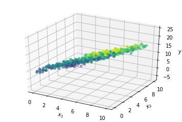
Ploting out data in 3D
from mpl_toolkits.mplot3d import Axes3D
fig = plt.figure()
ax = fig.add_subplot(111, projection="3d")
ax.scatter(X[:,0], X[:,1], y, c=y)
ax.set_xlabel("x_1")
ax.set_ylabel("x_2")
ax.set_zlabel("y")
Building our Linear Regression Model using Scikit Learn
from sklearn.linear_model import LinearRegression
lm = LinearRegression(fit_intercept=True)
lm.fit(X,y)
LinearRegression(copy_X=True, fit_intercept=True, n_jobs=1, normalize=False)
Evaluating Model
X_0 = np.array([2,4])
print("The predicted value is: ",lm.predict(X_0.reshape(1,-1)))
print("The accuracy is: ",lm.score(X, y))
The predicted value is:  [5.07289561]
The accuracy is:  0.9798997316600129
Assessing Model Accuracy
We can evaluate our model by spliting our data into two sets. One set is for training and another set is for testing. By using scikit learn library we can do it easily.
from sklearn.model_selection import train_test_split

X_train, X_test, y_train, y_test = train_test_split(X,y, train_size=0.5, random_state=1)
lm = LinearRegression(fit_intercept=True)
lm.fit(X_train, y_train)

print("Accuracy in test set: ",lm.score(X_test, y_test))
Accuracy in test set: 0.9794930834681773