What is NetworkX?

NetworkX is a Python package for the creation, manipulation, and study of the structure, dynamics, and functions of complex networks. It has powerful data structures for graphs, digraphs and multigraph and so on. You may refer to the reference to learn more about NetworkX

Many systems of scientific and societal interest consist of a large number of interacting components. The structure of these systems can be represented as networks where network nodes represent the components, and network edges, the interactions between the components. Network refers to the real world object, such as a road network, whereas a graph refers to its abstract mathematical representation. Graphs consist of nodes, also called vertices, and links, also called edges. Mathematically, a graph is a collection of vertices and edges where each edge corresponds to a pair of vertices. When we visualize graphs, we typically draw vertices as circles and edges as lines connecting the circles.

Get started with networkX

import networkx as nx
import matplotlib.pyplot as plt

# Creating an empty graph
G = nx.Graph()

# adding single node in graph
G.add_node("A")

# to add multiple nodes in graph
G.add_nodes_from(["B", "C", "D", "E", "F"])

# to display the nodes
G.nodes()

NodeView(('A', 'B', 'C', 'D', 'E', 'F'))

# to add edge between nodes
G.add_edge("A","B")

# to add multiple edges at a time
G.add_edges_from([("A","C"), ("A","D"), ("A","E"), ("E","F")])

# to view the edges
G.edges()

EdgeView([('A', 'B'), ('A', 'C'), ('A', 'D'), ('A', 'E'), ('E', 'F')])

# to know the number of edges
print(G.number_of_edges())

# to know the number of nodes
print(G.number_of_nodes())

5
6

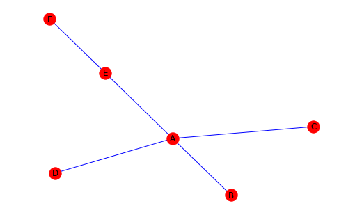
# We have created a graph with 5 nodes and 6 edges.
# Now let's view our graph.

nx.draw(G, with_labels=True, node_color="red", edge_color="blue")

# to remove node from graph
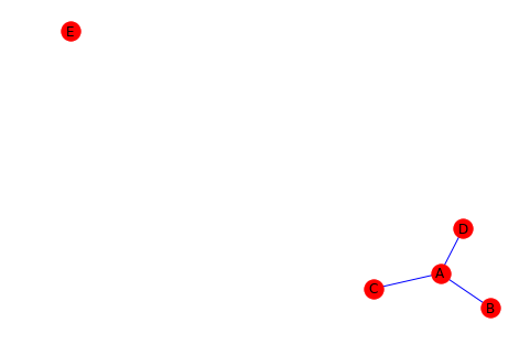
G.remove_node("F")

# to remove edge from graph
G.remove_edge("A","E")

# We can now visualize our graph after removing
# node F and edge A to E
nx.draw(G, with_labels=True, node_color="red", edge_color="blue")

Random Graph

The simplest possible random graph model is the so-called Erdos-Renyi, also known as the ER graph model. This family of random graphs has two parameters, capital N and lowercase p. Here the capital N is the number of nodes in the graph, and p is the probability for any pair of nodes to be connected by an edge. Here’s one way to think about it– imagine starting with N nodes and no edges. You can then go through every possible pair of nodes and with probability p insert an edge between them. In other words, you’re considering each pair of nodes once, independently of any other pair. You flip a coin to see if they’re connected, and then you move on to the next pair. If the value of p is very small, typical graphs generated from the model tend to be sparse, meaning having few edges. In contrast, if the value of p is large, typical graphs tend to be densely connected. Here we will implement our own ER model graph in order to learn and be able to create more complex graph by our own. We will use scipy bernoulli function for probability p.

The following steps can be taken to create our ER graph model

1. create an empty graph
2. add all n nodes in the graph
3. Loop over all pairs of nodes and add an edge wtih probability p

from scipy.stats import bernoulli

def er_graph(N, p):
    """ Generate an ER-Graph"""
    G = nx.Graph()
    G.add_nodes_from(range(N))
    for node1 in G.nodes():
        for node2 in G.nodes():
            if node1 < node2 and bernoulli.rvs(p=p):
                G.add_edge(node1, node2)
    return G

# lets call our er_graph model and visualize
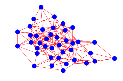
my_er_graph = er_graph(40, 0.2)
nx.draw(my_er_graph, node_color="blue", edge_color="red")

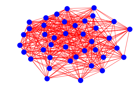
# if we increment the probalility the graph will be densly connected
nx.draw(er_graph(40, 0.5), node_color="blue", edge_color="red")

More Learning Resources

1. https://networkx.github.io/documentation/stable/tutorial.html
2. https://courses.edx.org/courses/course-v1:HarvardX+PH526x+2T2018/course/
3. https://docs.scipy.org/doc/scipy/reference/stats.html#discrete-distributions