Basic Concepts
# let's first import all the libraries needed for this tutorial

import pandas as pd
import numpy as np
import matplotlib.pyplot as plt
The primary data structures in pandas are implemented as two classes:
DataFrame, which you can imagine as a relational data table, with rows and named columns.
Series, which is a single column. A DataFrame contains one or more Series and a name for each Series.
day = ['Friday', 'Saturday', 'Sunday', 'Monday', 'Tuesday', 'Wednesday', 'Thursday' ]
first_sell = [100, 120, 310, 400, 90, 29, 30]
# to merge these two list we will use zip function
flower_sell = list(zip(day,first_sell))
[('Friday', 100),
 ('Saturday', 120),
 ('Sunday', 310),
 ('Monday', 400),
 ('Tuesday', 90),
 ('Wednesday', 29),
 ('Thursday', 30)]
# Great, we have created our dataset. Let's use pandas do some magic
df = pd.DataFrame(data = flower_sell, columns=['day', 'sell'] )
# df is for dataframe
|
day |
sell |
| 0 |
Friday |
100 |
| 1 |
Saturday |
120 |
| 2 |
Sunday |
310 |
| 3 |
Monday |
400 |
| 4 |
Tuesday |
90 |
| 5 |
Wednesday |
29 |
| 6 |
Thursday |
30 |
# we just have created pandas dataframe
# let's do similar with pandas series
day = pd.Series(['Friday', 'Saturday', 'Sunday', 'Monday', 'Tuesday', 'Wednesday', 'Thursday' ])
first_sell = pd.Series([100, 120, 310, 400, 90, 29, 30])
flower_sell = pd.DataFrame({'Day': day, 'Sell1': first_sell})
|
Day |
Sell1 |
| 0 |
Friday |
100 |
| 1 |
Saturday |
120 |
| 2 |
Sunday |
310 |
| 3 |
Monday |
400 |
| 4 |
Tuesday |
90 |
| 5 |
Wednesday |
29 |
| 6 |
Thursday |
30 |
# let's add another column for 2nd sell
flower_sell['Sell2'] = pd.Series([128, 230, 120, 231, 901, 140, 41])
|
Day |
Sell1 |
Sell2 |
| 0 |
Friday |
100 |
128 |
| 1 |
Saturday |
120 |
230 |
| 2 |
Sunday |
310 |
120 |
| 3 |
Monday |
400 |
231 |
| 4 |
Tuesday |
90 |
901 |
| 5 |
Wednesday |
29 |
140 |
| 6 |
Thursday |
30 |
41 |
accessing data
0    100
1    120
2    310
3    400
4     90
5     29
6     30
Name: Sell1, dtype: int64
0       Friday
1     Saturday
2       Sunday
3       Monday
4      Tuesday
5    Wednesday
6     Thursday
Name: Day, dtype: object
flower_sell['Sell2'][0:4]
0    128
1    230
2    120
3    231
Name: Sell2, dtype: int64
6     Thursday
5    Wednesday
4      Tuesday
3       Monday
2       Sunday
1     Saturday
0       Friday
Name: Day, dtype: object
Manipulating Data
flower_sell['Total_Sell'] = flower_sell['Sell1'] + flower_sell['Sell2']
|
Day |
Sell1 |
Sell2 |
Total_Sell |
| 0 |
Friday |
100 |
128 |
228 |
| 1 |
Saturday |
120 |
230 |
350 |
| 2 |
Sunday |
310 |
120 |
430 |
| 3 |
Monday |
400 |
231 |
631 |
| 4 |
Tuesday |
90 |
901 |
991 |
| 5 |
Wednesday |
29 |
140 |
169 |
| 6 |
Thursday |
30 |
41 |
71 |
# Now we can add another column as average sell
flower_sell['average_sell'] = flower_sell['Total_Sell']/2
|
Day |
Sell1 |
Sell2 |
Total_Sell |
average_sell |
| 0 |
Friday |
100 |
128 |
228 |
114.0 |
| 1 |
Saturday |
120 |
230 |
350 |
175.0 |
| 2 |
Sunday |
310 |
120 |
430 |
215.0 |
| 3 |
Monday |
400 |
231 |
631 |
315.5 |
| 4 |
Tuesday |
90 |
901 |
991 |
495.5 |
| 5 |
Wednesday |
29 |
140 |
169 |
84.5 |
| 6 |
Thursday |
30 |
41 |
71 |
35.5 |
# Let's save this file
flower_sell.to_csv('mysell', index='False',header='Small Business')
Indexes
Both Series and DataFrame objects also define an index property that assigns an identifier value to each Series item or DataFrame row.
By default, at construction, pandas assigns index values that reflect the ordering of the source data. Once created, the index values are stable; that is, they do not change when data is reordered.
RangeIndex(start=0, stop=7, step=1)
flower_sell.reindex([2, 6, 4])
|
Day |
Sell1 |
Sell2 |
Total_Sell |
average_sell |
| 2 |
Sunday |
310 |
120 |
430 |
215.0 |
| 6 |
Thursday |
30 |
41 |
71 |
35.5 |
| 4 |
Tuesday |
90 |
901 |
991 |
495.5 |
Working with large dataset
So far we have created a small dataframe and have done
some basic operation on it. Let’s work with large amount of
data. You can downlaod any dataset with google dataset search.
I have a csv file which I have donwloaded from www.kaggle.com
We will look into this and will perform some operation in it.
# First thing first, we need to read the file
# let's specify the location

location = r'C:\Users\ICT_H\Desktop\Machine Learning\File\train1.csv'
home_data = pd.read_csv(location)
# to describe the data we can do the following command
home_data.describe()
|
Id |
LotArea |
YearBuilt |
TotalBsmtSF |
BedroomAbvGr |
YrSold |
SalePrice |
| count |
1460.000000 |
1460.000000 |
1460.000000 |
1460.000000 |
1460.000000 |
1460.000000 |
1460.000000 |
| mean |
730.500000 |
10516.828082 |
1971.267808 |
1057.429452 |
2.866438 |
2007.815753 |
180921.195890 |
| std |
421.610009 |
9981.264932 |
30.202904 |
438.705324 |
0.815778 |
1.328095 |
79442.502883 |
| min |
1.000000 |
1300.000000 |
1872.000000 |
0.000000 |
0.000000 |
2006.000000 |
34900.000000 |
| 25% |
365.750000 |
7553.500000 |
1954.000000 |
795.750000 |
2.000000 |
2007.000000 |
129975.000000 |
| 50% |
730.500000 |
9478.500000 |
1973.000000 |
991.500000 |
3.000000 |
2008.000000 |
163000.000000 |
| 75% |
1095.250000 |
11601.500000 |
2000.000000 |
1298.250000 |
3.000000 |
2009.000000 |
214000.000000 |
| max |
1460.000000 |
215245.000000 |
2010.000000 |
6110.000000 |
8.000000 |
2010.000000 |
755000.000000 |
# to see only the first part of the dataset
home_data.head()
|
Id |
LotArea |
YearBuilt |
TotalBsmtSF |
BedroomAbvGr |
YrSold |
SaleType |
SalePrice |
| 0 |
1 |
8450 |
2003 |
856 |
3 |
2008 |
WD |
208500 |
| 1 |
2 |
9600 |
1976 |
1262 |
3 |
2007 |
WD |
181500 |
| 2 |
3 |
11250 |
2001 |
920 |
3 |
2008 |
WD |
223500 |
| 3 |
4 |
9550 |
1915 |
756 |
3 |
2006 |
WD |
140000 |
| 4 |
5 |
14260 |
2000 |
1145 |
4 |
2008 |
WD |
250000 |
# You can specify how many row you want to display. By default it's 5

home_data.head(10) # I want to display 10 raw
|
Id |
LotArea |
YearBuilt |
TotalBsmtSF |
BedroomAbvGr |
YrSold |
SaleType |
SalePrice |
| 0 |
1 |
8450 |
2003 |
856 |
3 |
2008 |
WD |
208500 |
| 1 |
2 |
9600 |
1976 |
1262 |
3 |
2007 |
WD |
181500 |
| 2 |
3 |
11250 |
2001 |
920 |
3 |
2008 |
WD |
223500 |
| 3 |
4 |
9550 |
1915 |
756 |
3 |
2006 |
WD |
140000 |
| 4 |
5 |
14260 |
2000 |
1145 |
4 |
2008 |
WD |
250000 |
| 5 |
6 |
14115 |
1993 |
796 |
1 |
2009 |
WD |
143000 |
| 6 |
7 |
10084 |
2004 |
1686 |
3 |
2007 |
WD |
307000 |
| 7 |
8 |
10382 |
1973 |
1107 |
3 |
2009 |
WD |
200000 |
| 8 |
9 |
6120 |
1931 |
952 |
2 |
2008 |
WD |
129900 |
| 9 |
10 |
7420 |
1939 |
991 |
2 |
2008 |
WD |
118000 |
# how about to look at the end of our dataset. We can do so by following

home_data.tail()
|
Id |
LotArea |
YearBuilt |
TotalBsmtSF |
BedroomAbvGr |
YrSold |
SaleType |
SalePrice |
| 1455 |
1456 |
7917 |
1999 |
953 |
3 |
2007 |
WD |
175000 |
| 1456 |
1457 |
13175 |
1978 |
1542 |
3 |
2010 |
WD |
210000 |
| 1457 |
1458 |
9042 |
1941 |
1152 |
4 |
2010 |
WD |
266500 |
| 1458 |
1459 |
9717 |
1950 |
1078 |
2 |
2010 |
WD |
142125 |
| 1459 |
1460 |
9937 |
1965 |
1256 |
3 |
2008 |
WD |
147500 |
# we can visualize particular column as well

home_data.hist('SalePrice')
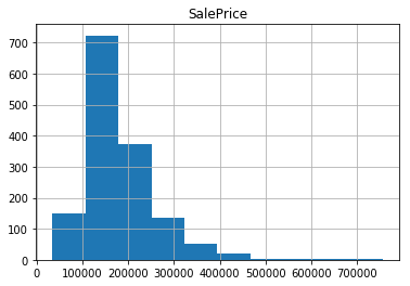
saleprice = home_data['SalePrice']
NumPy is a popular toolkit for scientific computing. pandas Series can be used as arguments to most NumPy functions:
np.log(saleprice) # to get the logarithmic value of salaprice
0       12.247694
1       12.109011
2       12.317167
3       11.849398
4       12.429216
5       11.870600
6       12.634603
7       12.206073
8       11.774520
9       11.678440
10      11.771436
11      12.751300
12      11.877569
13      12.540758
14      11.964001
15      11.790557
16      11.911702
17      11.407565
18      11.976659
19      11.842229
20      12.692503
21      11.845103
22      12.345835
23      11.774520
24      11.944708
25      12.454104
26      11.811547
27      12.631340
28      12.242887
29      11.134589
          ...
1430    12.165980
1431    11.875831
1432    11.074421
1433    12.136187
1434    11.982929
1435    12.066811
1436    11.699405
1437    12.885671
1438    11.916389
1439    12.190959
1440    12.160029
1441    11.913713
1442    12.644328
1443    11.703546
1444    12.098487
1445    11.767568
1446    11.969717
1447    12.388394
1448    11.626254
1449    11.429544
1450    11.820410
1451    12.567551
1452    11.884489
1453    11.344507
1454    12.128111
1455    12.072541
1456    12.254863
1457    12.493130
1458    11.864462
1459    11.901583
Name: SalePrice, Length: 1460, dtype: float64
saleprice.apply(lambda val: val > 100000)
0        True
1        True
2        True
3        True
4        True
5        True
6        True
7        True
8        True
9        True
10       True
11       True
12       True
13       True
14       True
15       True
16       True
17      False
18       True
19       True
20       True
21       True
22       True
23       True
24       True
25       True
26       True
27       True
28       True
29      False
        ...
1430     True
1431     True
1432    False
1433     True
1434     True
1435     True
1436     True
1437     True
1438     True
1439     True
1440     True
1441     True
1442     True
1443     True
1444     True
1445     True
1446     True
1447     True
1448     True
1449    False
1450     True
1451     True
1452     True
1453    False
1454     True
1455     True
1456     True
1457     True
1458     True
1459     True
Name: SalePrice, Length: 1460, dtype: bool
Dealing with missing data
Let’s create a pandas dataframe with missing data
name = pd.Series(['a', 'b', 'c', 'd', 'e', 'f'])
price = pd.Series([10, 20, 15])
missing_data = pd.DataFrame({'Name': name, 'Price': price})
|
Name |
Price |
| 0 |
a |
10.0 |
| 1 |
b |
20.0 |
| 2 |
c |
15.0 |
| 3 |
d |
NaN |
| 4 |
e |
NaN |
| 5 |
f |
NaN |
missing_data['Price'].isna()
0    False
1    False
2    False
3     True
4     True
5     True
Name: Price, dtype: bool
# we can fill missing values with: fillna() method
missing_data['Price'].fillna(0) # to fill with 0
0    10.0
1    20.0
2    15.0
3     0.0
4     0.0
5     0.0
Name: Price, dtype: float64
missing_data['Price'].fillna('missing')
0         10
1         20
2         15
3    missing
4    missing
5    missing
Name: Price, dtype: object
We can’t build model with missing value. There are several ways
to deal with missing value while building model. I will discuss about
it in my future post.
If you want to learn more about pandas: visit: https://pandas.pydata.org/pandas-docs/stable/cookbook.html#missing-data