Numpy array
NumPy’s main object is the homogeneous multidimensional array. It is a table of elements (usually numbers), all of the same type, indexed by a tuple of positive integers. In NumPy dimensions are called axes.
For example, the coordinates of a point in 3D space [1, 2, 1] has one axis. That axis has 3 elements in it, so we say it has a length of 3. In the example pictured below, the array has 2 axes. The first axis has a length of 2, the second axis has a length of 3.
[[1., 0., 0.],
 [0., 1., 2.]]
NumPy’s array class is called ndarray. It is also known by the alias array. Note that numpy.array is not the same as the Standard Python Library class array.array, which only handles one-dimensional arrays and offers less functionality. The more important attributes of an ndarray object are:
ndarray.ndim the number of axes (dimensions) of the array.
ndarray.shape the dimensions of the array. This is a tuple of integers indicating the size of the array in each dimension. For a matrix with n rows and m columns, shape will be (n,m). The length of the shape tuple is therefore the number of axes, ndim.
ndarray.size => the total number of elements of the array. This is equal to the product of the elements of shape.
ndarray.dtype an object describing the type of the elements in the array. One can create or specify dtype’s using standard Python types. Additionally NumPy provides types of its own. numpy.int32, numpy.int16, and numpy.float64 are some examples.
import numpy as np
a = np.arange(18).reshape(3,6)
a
array([[ 0,  1,  2,  3,  4,  5],
       [ 6,  7,  8,  9, 10, 11],
       [12, 13, 14, 15, 16, 17]])
a.shape
(3, 6)
a.ndim
2
a.dtype
dtype('int32')
a.size
18
Array Creation
There are several ways to create arrays.
For example, you can create an array from a regular Python list or tuple using the array function. The type of the resulting array is deduced from the type of the elements in the sequences.
b = np.array([4,5,3])
b
array([4, 5, 3])
array transforms sequences of sequences into two-dimensional arrays, sequences of sequences of sequences into three-dimensional arrays, and so on.
c = np.array([(1,3,6), (4,9,2)])
c
array([[1, 3, 6],
       [4, 9, 2]])
Often, the elements of an array are originally unknown, but its size is known. Hence, NumPy offers several functions to create arrays with initial placeholder content. These minimize the necessity of growing arrays, an expensive operation.
The function zeros creates an array full of zeros, the function ones creates an array full of ones, and the function empty creates an array whose initial content is random and depends on the state of the memory. By default, the dtype of the created array is float64.
np.zeros((3,4))
array([[0., 0., 0., 0.],
       [0., 0., 0., 0.],
       [0., 0., 0., 0.]])
np.ones((4,4))
array([[1., 1., 1., 1.],
       [1., 1., 1., 1.],
       [1., 1., 1., 1.],
       [1., 1., 1., 1.]])
np.empty((2,3))
array([[0., 0., 0.],
       [0., 0., 0.]])
To create sequences of numbers, NumPy provides a function analogous to range that returns arrays instead of lists.
np.arange(10, 30, 5)
array([10, 15, 20, 25])
When arange is used with floating point arguments, it is generally not possible to predict the number of elements obtained, due to the finite floating point precision. For this reason, it is usually better to use the function linspace that receives as an argument the number of elements that we want, instead of the step:
np.linspace( 0, 2, 9)
array([0. , 0.25, 0.5 , 0.75, 1. , 1.25, 1.5 , 1.75, 2. ])
x = np.linspace(2, 20, 15)
y = x**2
x
array([ 2.        ,  3.28571429,  4.57142857,  5.85714286,  7.14285714,
        8.42857143,  9.71428571, 11.        , 12.28571429, 13.57142857,
       14.85714286, 16.14285714, 17.42857143, 18.71428571, 20.        ])
y
array([  4.        ,  10.79591837,  20.89795918,  34.30612245,
        51.02040816,  71.04081633,  94.36734694, 121.        ,
       150.93877551, 184.18367347, 220.73469388, 260.59183673,
       303.75510204, 350.2244898 , 400.        ])
linspace function is very useful it you want evaluate a function in many different point.
Arithmetic operators on arrays apply elementwise. A new array is created and filled with the result.
e = np.array([5, 3, 6, 8])
f = np.array([2, 1, 4, 9])
g = e - f
g
array([ 3, 2, 2, -1])
g > 0
array([ True, True, True, False])
Unlike in many matrix languages, the product operator * operates elementwise in NumPy arrays. The matrix product can be performed using the @ operator (in python >=3.5) or the dot function or method:
e * f # elementwise product
array([10, 3, 24, 72])
e @ f # matrix product
109
e.dot(f) # another matrix product
109
Indexing Slicing and Iterating
One-dimensional arrays can be indexed, sliced and iterated over, much like lists and other Python sequences.
g = np.arange(2, 10)
g
array([2, 3, 4, 5, 6, 7, 8, 9])
g[3:5]
array([5, 6])
g[::-1]
array([9, 8, 7, 6, 5, 4, 3, 2])
h = np.array([[3,4,5],[7,8,9]])
h[1,1]
8
Iterating over multidimensional arrays is done with respect to the first axis:
for row in h:
    print(row)
[3 4 5]
[7 8 9]
An array has a shape given by the number of elements along each axis:
i = np.arange(2, 20).reshape(3,6)
i
array([[ 2,  3,  4,  5,  6,  7],
       [ 8,  9, 10, 11, 12, 13],
       [14, 15, 16, 17, 18, 19]])
The shape of an array can be changed with various commands. Note that the following three commands all return a modified array, but do not change the original array:
i.ravel() # return the array flattened
array([ 2,  3,  4,  5,  6,  7,  8,  9, 10, 11, 12, 13, 14, 15, 16, 17, 18,
       19])
i.reshape(2,9) # return the array in different shape
array([[ 2,  3,  4,  5,  6,  7,  8,  9, 10],
       [11, 12, 13, 14, 15, 16, 17, 18, 19]])
i.T # return the array , transposed
array([[ 2,  8, 14],
       [ 3,  9, 15],
       [ 4, 10, 16],
       [ 5, 11, 17],
       [ 6, 12, 18],
       [ 7, 13, 19]])
i.T.shape
(6, 3)
i.shape
(3, 6)
Copies and Views
When operating and manipulating arrays, their data is sometimes copied into a new array and sometimes not. This is often a source of confusion for beginners. There are three cases:
1. No copy at all
Simple assignment make no copy of array objects or of their data
j = np.arange(3,4)
k = j # no new object created
k is j # j, k are two names for smae ndarray object
True
2. View or Shallow Copy
Different array objects can share the same data. The view method creates a new array object that looks at the same data.
l = j.view()
l is j # l is new different object
False
l.base is j # l is view of j
True
3. Deep Copy
The copy method makes a complete copy of the array and its data
m = j.copy() # complete deep copy new object wit same data but not sharing
m is j
False
m.base is j
False